The out-of-the-box dbt snapshots provide change data capture (CDC) capability for tracking the changes to data in your data lake or data warehouse. The dbt snapshot metadata columns enable a view of change to data - which records have been updated and when. However, the dbt snapshot metadata doesn't provide a view of the processing audit - which process or job was responsible for the changes. The ability to audit at the processing level requires additional operational metadata.

The out-of-the-box dbt snapshot strategies (rules for detecting changes) likely provide the desired logic for detecting and managing data change. No change to the snapshot strategies or snapshot pipeline processing is desired, but additional operational metadata fields must be set and carried through with the data.

Objectives​

Both operational and governance requirements can drive the need for greater fidelity of operational metadata. Example considerations could include:

• use of the out-of-the-box dbt snapshot logic and strategies for Change Data Capture (CDC)
• addition of operational metadata fields to snapshot tables with processing details for ops support and audit
  • when new records are inserted, add operational processing metadata information to each record
  • when existing records are closed or end-dated, update operational metadata fields with processing metadata

Aside from including a new process_id value in records, these enhancements don't add further information to the table. Instead they are a materialization of the operational data that is easier to access. The same information could be derived from standard dbt metadata fields but would require a more complex SQL statement that includes a left outer self-join. As with any materialization decision, there is a trade-off between ease of access vs. additional storage requirements.

NULL vs High-End Date/Timestamp​

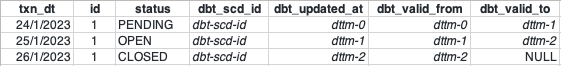
In addition to the ops support and audit requirements, there can also be a legacy migration complication related to how open records (the most current version of the record) are represented in snapshots. dbt snapshots represent open records using NULL values for dbt_valid_to fields. In legacy data lakes or data warehouses, the open records often are identified using a well-known high value for the effective end date/timestamp, such as 9999-12-31 or 9999-12-31 23:59:59. Adding additional snapshot metadata columns enables a legacy view of record changes without having to alter the dbt snapshot strategy or processing logic.

datetime('9999-12-31 23:59:59.999999', 'Australia/Melbourne')

timestamp('9999-12-31 23:59:59.999999', 'Australia/Melbourne')

Enhancing the default Snapshot​

Modify the default dbt snapshot behavior by overriding the dbt snapshot materialization macros. dbt enbles macros to be overridden using the following resolution or search order:

1. locally defined macros in the project's ./macros directory
2. macros defined in additional dbt packages included in the project packages.yml file
3. dbt adaptor-specific macros
4. dbt provided default macros

To inject additional snapshot metadata fields into snapshot tables override the following two default macros:

• default__build_snapshot_table() creates the snapshot table on the first run
• default__snapshot_staging_table() stages in the inserts and updates to be applied to the snapshot table

To update fields on snapshot update, override the following default macro:

• default__snapshot_merge_sql() performs the MERGE/UPSERT

Note that if the dbt database adaptor implements adaptor-specific versions of these macros, then update the adaptor-specific macro accordingly. For example the dbt-spark adaptor overrides the dbt default__snapshot_merge_sql() as spark__snapshot_merge_sql().

build_snapshot_table()​

The default__build_snapshot_table() macro is called on the first dbt snapshot invocation. This macro defines the content to include in the CREATE TABLE statement. The following example adds process id's using the dbt invocation_id and additional timestamp fields, including use of the well-known high timestamp value for open records. This value is defined as the variable default_high_dttm in the dbt_project.yml file. The dbt snapshot strategy processing uses the unmodified standard dbt columns, so modification to change detection logic is not required.

snapshot_staging_table()​

The default__snapshot_staging_table() macro is called on subsequent dbt snapshot invocations. This macro defines the content in the MERGE statement for inserts and updates. The following example adds the additional operational metadata fields to the insertions common table expression (CTE) and the updates (CTE). The dbt invocation_id is used again as the process_id for inserts on new records and updates that close existing records.

Note that the deletes CTE has not been updated with the additional fields. In scenarios that use the hard deletes feature, the deletes CTE would need to be modified as well.

snapshot_merge_sql()​

The default__snapshot_merge_sql() macro is called to perform the MERGE/UPSERT into the target snapshot table. This macro defines how fields in the records being closed should be updated. The update set section of the MERGE statement defines the updated columns and values.

Conclusion​

Overriding the default dbt snapshot macros enables the injection and updating of additional operational metadata in snapshot tables. Fields can be added such that the provided dbt logic and snapshot strategy processing is still applied. Still, the resulting snapshot tables contain the columns required for the data lake or data warehouse.

The sample dbt project in datwiz/dbt-snapshot-metadata/tree/main/dbt_snapshot_ops_metadata contains an implementation of the snapshot customization.

DBT (or Data Build Tool) is a modern data transformation tool born in the cloud/DevOps era. It's a great project which much has been written about; I will try to give as brief an overview as possible.

ETL vs ELT Refresher

A quick refresher on ELT vs ETL before we discuss DBT. I have created an infographic for this...

Summary​

DBT is an open-source command line tool written in Python from DBT Labs (formerly Fishtown Analytics).

DBT is designed to manage data transformations while applying software engineering best practices (including version control, automated testing, reviews, approvals, etc). Its modern software engineering and cloud-first design goals separate it from its old-school ETL/ELT predecessors.

DBT is an ELT tool focusing on the T(ransform) only, the E(xtract) and L(oad) are up to you (there are plenty of tools that specialize in this).

At its core DBT is a templating engine using Jinja (Python templating engine); it generates templates that represent SQL commands to create, replace or update objects in your database (the “T” in ELT), then oversees the execution of the templated commands. The work is "pushed down" to the underlying database containing the source and target objects and data.

Models​

The concept most integral to DBT is the Model. A Model is simply a representation of a transform (or set of transforms) to a dataset, resulting in a target object (which could be a table or tables in a datamart). A model is expressed as a SELECT statement stored in a .sql file in your dbt project (well get to that in a minute).

Suppose we want to create a denormalized fact table for commits to store in a datamart in BigQuery. This is what a model file might look like (using the BigQuery SQL dialect and referencing objects that should exist and be accessible at runtime when we execute the model).

{{ config(materialized='table') }}

with commits as (
    SELECT 
    SUBSTR(commit, 0, 13) as commit_short_sha,
    committer.name as commiter_name,
    committer.date as commit_date,
    message,
    repo_name
    FROM `bigquery-public-data.github_repos.sample_commits` c
)

select * from commits

Models are created as views by default, but you can materialize these as tables where needed.

You configure connectivity to the target database using adapters (software libraries provided by dbt in the case of most mainstream databases) and profiles (which contain details around authentication, databases/datasets, schemas etc).

DBT Project​

A DBT project is simply a folder containing your models and some other configuration data. You can initialize this by running dbt init from your desired project directory. In its most basic form, the structure looks like this:

models/
├─ your_model.sql
├─ schema.yml
dbt_project.yml

Your models can be created under subfolders for organization. schema.yml is an optional file that contains tests for columns, can also include descriptions for documentation. The dbt_project.yml file is the main entry point for the dbt program, it contains the configuration for the project, including which profile to use. Profiles (stored in a file called profiles.yml store all of the necessary connectivity information for your target database platform. By default dbt init creates this file a .dbt folder under your home directory.

To confirm your project is ship shape, run dbt parse; if there are no errors, you are good to proceed running and testing your models.

Running DBT Models​

To run your models, simply run the following command from the directory containing your dbt_project.yml file (typically the root of your project folder):

dbt run

06:56:36  Running with dbt=1.2.0
06:56:36  Found 1 model, 2 tests, 0 snapshots, 0 analyses, 285 macros, 0 operations, 0 seed files, 0 sources, 0 exposures, 0 metrics
06:56:36
06:56:37  Concurrency: 1 threads (target='dev')
06:56:37
06:56:37  1 of 1 START table model dbt_dataset.fct_commits ............................... [RUN]
06:56:50  1 of 1 OK created table model dbt_dataset.fct_commits .......................... [CREATE TABLE (672.3k rows, 396.7 MB processed) in 13.28s]
06:56:50
06:56:50  Finished running 1 table model in 0 hours 0 minutes and 14.01 seconds (14.01s).
06:56:50
06:56:50  Completed successfully
06:56:50
06:56:50  Done. PASS=1 WARN=0 ERROR=0 SKIP=0 TOTAL=1

Model deployed! Let's test it:

dbt test

06:57:19  Running with dbt=1.2.0
06:57:19  Found 1 model, 2 tests, 0 snapshots, 0 analyses, 285 macros, 0 operations, 0 seed files, 0 sources, 0 exposures, 0 metrics
06:57:19
06:57:19  Concurrency: 1 threads (target='dev')
06:57:19
06:57:19  1 of 2 START test not_null_fct_commits_commit_short_sha ........................ [RUN]
06:57:21  1 of 2 PASS not_null_fct_commits_commit_short_sha .............................. [PASS in 1.88s]
06:57:21  2 of 2 START test unique_fct_commits_commit_short_sha .......................... [RUN]
06:57:24  2 of 2 PASS unique_fct_commits_commit_short_sha ................................ [PASS in 3.14s]
06:57:24
06:57:24  Finished running 2 tests in 0 hours 0 minutes and 5.41 seconds (5.41s).
06:57:24
06:57:24  Completed successfully
06:57:24
06:57:24  Done. PASS=2 WARN=0 ERROR=0 SKIP=0 TOTAL=2

This will run all of the tests associated with your model(s) - in this case, not null and unique tests defined in the schema.yml file. That's it, deployed and tested.

Other Stuff​

There is some other stuff in DBT you should be aware of, like seeds, snapshots, analyses, macros, and more but our five minutes is up 😃. We can discuss these next time; you are up and running with the basics of DBT now, get transforming!

if you have enjoyed this post, please consider buying me a coffee ☕ to help me keep writing!

Loading Parquet format files into BigQuery is straightforward, you just need to specify the file location (local, Google Cloud Storage, Drive, Amazon S3 or Azure Blob storage) and thats pretty much it, BigQuery works the rest out from there.

bq load \
--location=australia-southeast2 \
--project_id=parquet-demo \
--source_format=PARQUET \
parquet_test.dim_calendar \
.\Calendar.gzip

In Snowflake, however, it is not as simple, I'll share my approach to automating this here.

Background​

Data in a Parquet file is stored in a single column for a self-contained dataset. If you were to ingest this into Snowflake without knowing the schema you could do something like this...

CREATE OR REPLACE TABLE PARQUET_TEST.PUBLIC.DIM_CALENDAR (
  Data variant
);

COPY INTO PARQUET_TEST.PUBLIC.DIM_CALENDAR 
(
  Data
) FROM (
SELECT
*
FROM
@PARQUET_TEST.PUBLIC.DIM_CALENDAR_STAGE)
  file_format = (TYPE = parquet);

You would end up with something like...

You could then have a second stage of processing to convert this into a normal relational structure.

Or you could do this in one step, with a little prep work ahead of time. In my scenario I was given several parquet files from a client for a one-off load into Snowflake, several files for a fact table and multiple single files representing different dimension tables.

Streamlined Ingestion for Parquet Files into Snowflake​

To collapse the formatting and uploading of Parquet files into a materialized table into one step, we need to do a couple of things:

1. Create the target table with the correct schema (column names and data types); and
2. perform a projection in our COPY command from the single column containing all of the data (represented by $1 in Snowflake) into columns defined in step 1

Since this is technically a transformation and only named stages are supported for COPY transformations, we need to create a stage for the copy. In my case there is a pre-existing Storage Integration in place that can be used by the stage.

Generate Table DDL​

To automate the generation of the DDL to create the table and stage and the COPY command, I used Python and Spark (which has first class support for Parquet files). Parquet datatypes are largely the same as Snowflake, but if we needed to, we could create a map and modify the target types during the DDL generation.

First copy specimen Parquet formatted files to a local directory, the script we are creating can then iterate through the parquet files and generate all of the commands we will need saved to a .sql file.

With some setup information provided (not shown for brevity), we will first go through each file in the directory, capture metadata along with the schema (column name and data type) as shown here:

for file in files:
    tableMap = {}
    table = file.stem
    spark = launch_spark_session()
    parquetFile = spark.read.parquet("%s/%s" %(BASE_DIR, file))
    data_types = parquetFile.dtypes
    stop_spark_session(spark)
    tableMap['name'] = table
    tableMap['file'] = file
    tableMap['data_types'] = data_types
    allTables.append(tableMap)

The allTables list looks something like this...

[{'name': 'Calendar', 'file': PosixPath('data/dim/Calendar.gzip'), 'data_types': [('Time_ID', 'bigint'), ('CalYear', 'bigint'), ('CalMonthOfYearNo', 'bigint'), ('FinYear', 'bigint'), ('FinWeekOfYearNo', 'bigint')]}, ... ]

Next we generate the CREATE TABLE statement using the allTables list:

# create output file for all sql
with open('all_tables.sql', 'w') as f:
    for table in allTables:
        print("processing %s..." % table['name'])
        f.write("/*** Create %s Table***/" % table['name'].upper())
        sql = """
CREATE OR REPLACE TABLE %s.%s.%s (
""" % (database, schema, table['name'].upper())
        for column in table['data_types']:
            sql += "  %s %s,\n" % (column[0], column[1])
        sql = sql[:-2] + "\n);"
        f.write(sql)
        f.write("\n\n")

Generate Named Stage DDL​

Then we generate the stage in S3 from which the files will be loaded:

        f.write("/*** Create %s Stage***/" % table['name'].upper())
        sql = """
CREATE OR REPLACE STAGE %s.%s.%s_STAGE 
  url='%s/%s'
  storage_integration = %s
  encryption=(type='AWS_SSE_KMS' kms_key_id = '%s');
""" % (database, schema, table['name'].upper(), s3_prefix, table['file'], storage_int, kms_key_id)
        f.write(sql)
        f.write("\n\n")

Generate COPY commands​

Then we generate the COPY commands...

        f.write("/*** Copying Data into %s ***/" % table['name'].upper())
        sql = """
COPY INTO %s.%s.%s 
(\n""" % (database, schema, table['name'].upper())
        for column in table['data_types']:
            sql += "  %s,\n" % column[0]
        sql = sql[:-2] + "\n)"
        sql += " FROM (\nSELECT\n"
        for column in table['data_types']:
            sql += "  $1:%s::%s,\n" % (column[0], column[1])
        sql = sql[:-2] + "\nFROM\n"
        sql += "@%s.%s.%s_STAGE)\n" % (database, schema, table['name'].upper()) 
        sql += "  file_format = (TYPE = parquet);"
        f.write(sql)
        f.write("\n\n")

Since this is a one off load, we will go ahead and drop the stage we created as it is no longer needed (this step is optional)..

        f.write("/*** Dropping stage for %s ***/" % table['name'].upper())
        sql = """
DROP STAGE %s.%s.%s_STAGE; 
""" % (database, schema, table['name'].upper())
        f.write(sql)
        f.write("\n\n")

The resultant file created looks like this..

/*** Create CALENDAR Table***/
CREATE OR REPLACE TABLE PARQUET_TEST.PUBLIC.DIM_CALENDAR (
  Time_ID bigint,
  CalYear bigint,
  CalMonthOfYearNo bigint,
  FinYear bigint,
  FinWeekOfYearNo bigint
);

/*** Create DIM_CALENDAR Stage***/
CREATE OR REPLACE STAGE PARQUET_TEST.PUBLIC.DIM_CALENDAR_STAGE 
  url='s3://my-bucket/data/dim/Calendar.gzip'
  storage_integration = my_storage_int
  encryption=(type='AWS_SSE_KMS' kms_key_id = '4f715ec9-ee8e-44ab-b35d-8daf36c05f19');

/*** Copying Data into DIM_CALENDAR ***/
COPY INTO PARQUET_TEST.PUBLIC.DIM_CALENDAR 
(
  Time_ID,
  CalYear,
  CalMonthOfYearNo,
  FinYear,
  FinWeekOfYearNo
) FROM (
SELECT
  $1:Time_ID::bigint,
  $1:CalYear::bigint,
  $1:CalMonthOfYearNo::bigint,
  $1:FinYear::bigint,
  $1:FinWeekOfYearNo::bigint
FROM
@PARQUET_TEST.PUBLIC.DIM_CALENDAR_STAGE)
  file_format = (TYPE = parquet);

/*** Dropping stage for DIM_CALENDAR ***/
DROP STAGE PARQUET_TEST.PUBLIC.DIM_CALENDAR_STAGE; 

Load your data​

You can then run this along with all of the other dimension and fact table DDL and COPY commands generated to perform the one-off load from parquet files. You can find the complete code below, enjoy!

from pathlib import Path
from pyspark.sql import SparkSession

def launch_spark_session():
    return SparkSession \
        .builder \
        .appName("Parquet DDL Generation") \
        .getOrCreate()

def stop_spark_session(spark):
    spark.stop()

allTables = []
database = "PARQUET_TEST" 
schema = "PUBLIC"
s3_prefix = 's3://my-bucket'
storage_int = 'my_storage_int'
kms_key_id = '4f715ec9-ee8e-44ab-b35d-8daf36c05f19'

BASE_DIR = Path(__file__).resolve().parent
directory = 'data/dim'
files = Path(directory).glob('*.gzip')
for file in files:
    tableMap = {}
    table = file.stem
    spark = launch_spark_session()
    parquetFile = spark.read.parquet("%s/%s" %(BASE_DIR, file))
    data_types = parquetFile.dtypes
    stop_spark_session(spark)
    tableMap['name'] = table
    tableMap['file'] = file
    tableMap['data_types'] = data_types
    allTables.append(tableMap)

# create output file for all sql
with open('all_tables.sql', 'w') as f:
    for table in allTables:
        print("processing %s..." % table['name'])
        f.write("/*** Create %s Table***/" % table['name'].upper())
        sql = """
CREATE OR REPLACE TABLE %s.%s.%s (
""" % (database, schema, table['name'].upper())
        for column in table['data_types']:
            sql += "  %s %s,\n" % (column[0], column[1])
        sql = sql[:-2] + "\n);"
        f.write(sql)
        f.write("\n\n")
        
        f.write("/*** Create %s Stage***/" % table['name'].upper())
        sql = """
CREATE OR REPLACE STAGE %s.%s.%s_STAGE 
  url='%s/%s'
  storage_integration = %s
  encryption=(type='AWS_SSE_KMS' kms_key_id = '%s');
""" % (database, schema, table['name'].upper(), s3_prefix, table['file'], storage_int, kms_key_id)
        f.write(sql)
        f.write("\n\n")

        f.write("/*** Copying Data into %s ***/" % table['name'].upper())
        sql = """
COPY INTO %s.%s.%s 
(\n""" % (database, schema, table['name'].upper())
        for column in table['data_types']:
            sql += "  %s,\n" % column[0]
        sql = sql[:-2] + "\n)"
        sql += " FROM (\nSELECT\n"
        for column in table['data_types']:
            sql += "  $1:%s::%s,\n" % (column[0], column[1])
        sql = sql[:-2] + "\nFROM\n"
        sql += "@%s.%s.%s_STAGE)\n" % (database, schema, table['name'].upper()) 
        sql += "  file_format = (TYPE = parquet);"
        f.write(sql)
        f.write("\n\n")

        f.write("/*** Dropping stage for %s ***/" % table['name'].upper())
        sql = """
DROP STAGE %s.%s.%s_STAGE; 
""" % (database, schema, table['name'].upper())
        f.write(sql)
        f.write("\n\n")

if you have enjoyed this post, please consider buying me a coffee ☕ to help me keep writing!

It is common to have a remote and dispersed team these days. As face to face meetings are less common and with geographically dispersed development teams not possible, it is challenging to have a clear picture of where your team is.

GitHub provides useful data to help us understand your development team's workload and progress. StackQL has an official GitHub provider which allows you to access this data using SQL.

In this example we will use the pystackql Python package (Python wrapper for StackQL) along with a Jupyter Notebook to retrieve data from GitHub using SQL, then sink the data into a cloud native data warehouse for long term storage and analytics at scale, in this example we have used BigQuery.

Step by Step Guide​

This guide will walk you through the steps involved in capturing and analyzing developer data using StackQL, Python, Jupyter and BigQuery.

1. Create GitHub Personal Access Token​

You will need to create a Personal Access Token in GitHub for a user which has access to the org or orgs in GitHub you will be analyzing. Follow this guide to create your GitHub token and store it somewhere safe.

2. Setup your Jupyter Notebook​

You need to set up your Jupyter environment, you can either use the Docker, see stackql/stackql-jupyter-demo or:

1. Create your Jupyter project
2. Download and install StackQL
3. Clone the pystackql repo

3. Setup StackQL Authentication to GitHub​

You can find instructions on how to use your personal access token to authenticate to GitHub here. The following example shows how to do this in a Jupyter notebook cell using pystackql.

4. Retrieve data​

Next, we will use StackQL SQL queries to get commits, pull requests and pull request reviews, then we will aggregate by usernames of contributors. You can use JOIN semantics in StackQL to do this as well.

Get Contributors, Commits, Pull Requests and Reviews​

In the following cell we will query data from GitHub using StackQL:

Aggregate Data By Username​

Now we will aggregate the data by each contributor, see the following example:

5. Store the Data in BigQuery​

After the transformation of data, we will then upload it to BigQuery. First, we will store the data as a new line delimited json file, making the uploading process much easier and handling the nested schema better, as shown in the following cell:

Now we can see the table on BigQuery as shown here:

From here you can use the same process to append data to the table and use BigQuery to perform analytics at scale on the data.

So you're using BigQuery (BQ). It's all set up and humming perfectly. Maybe now, you want to run an ELT job whenever a new table partition is created, or maybe you want to retrain your ML model whenever new rows are inserted into the BQ table.

In my previous article on EventArc, we went through how Logging can help us create eventing-type functionality in your application. Let's take it a step further and walk through how we can couple BigQuery and Cloud Run.

In this article you will learn how to

• Tie together BigQuery and Cloud Run
• Use BigQuery's audit log to trigger Cloud Run
• With those triggers, run your required code

Let's go!​

Let's create a temporary dataset within BigQuery named tmp_bq_to_cr.

In that same dataset, let's create a table in which we will insert some rows to test our BQ audit log. Let's grab some rows from a BQ public dataset to create this table:

CREATE OR REPLACE TABLE tmp_bq_to_cr.cloud_run_trigger AS
SELECT
 date, country_name, new_persons_vaccinated, population
 from `bigquery-public-data.covid19_open_data.covid19_open_data`
 where country_name='Australia'
 AND
 date > '2021-05-31'
LIMIT 100

Following this, let's run an insert query that will help us build our mock database trigger:

INSERT INTO tmp_bq_to_cr.cloud_run_trigger
VALUES('2021-06-18', 'Australia', 3, 1000)

Now, in another browser tab let's navigate to BQ Audit Events and look for our INSERT INTO event:

There will be several audit logs for any given BQ action. Only after a query is parsed does BQ know which table we want to interact with, so the initial log will, for e.g., not have the table name.

We don't want any old audit log, so we need to ensure we look for a unique set of attributes that clearly identify our action, such as in the diagram above.

In the case of inserting rows, the attributes are a combination of

• The method is google.cloud.bigquery.v2.JobService.InsertJob
• The name of the table being inserted to is the protoPayload.resourceName
• The dataset id is available as resource.labels.dataset_id
• The number of inserted rows is protoPayload.metadata.tableDataChanged.insertedRowsCount

Time for some code​

Now that we've identified the payload that we're looking for, we can write the action for Cloud Run. We've picked Python and Flask to help us in this instance. (full code is on GitHub).

First, let's filter out the noise and find the event we want to process

@app.route('/', methods=['POST'])
def index():
    # Gets the Payload data from the Audit Log
    content = request.json
    try:
        ds = content['resource']['labels']['dataset_id']
        proj = content['resource']['labels']['project_id']
        tbl = content['protoPayload']['resourceName']
        rows = int(content['protoPayload']['metadata']
                   ['tableDataChange']['insertedRowsCount'])
        if ds == 'cloud_run_tmp' and \
           tbl.endswith('tables/cloud_run_trigger') and rows > 0:
            query = create_agg()
            return "table created", 200
    except:
        # if these fields are not in the JSON, ignore
        pass
    return "ok", 200

Now that we've found the event we want, let's execute the action we need. In this example, we'll aggregate and write out to a new table created_by_trigger:

def create_agg():
    client = bigquery.Client()
    query = """
    CREATE OR REPLACE TABLE tmp_bq_to_cr.created_by_trigger AS
    SELECT
      count_name, SUM(new_persons_vaccinated) AS n
    FROM tmp_bq_to_cr.cloud_run_trigger
    """
    client.query(query)
    return query

The Dockerfile for the container is simply a basic Python container into which we install Flask and the BigQuery client library:

FROM python:3.9-slim
RUN pip install Flask==1.1.2 gunicorn==20.0.4 google-cloud-bigquery
ENV APP_HOME /app
WORKDIR $APP_HOME
COPY *.py ./
CMD exec gunicorn --bind :$PORT main:app

Now we Cloud Run​

Build the container and deploy it using a couple of gcloud commands:

SERVICE=bq-cloud-run
PROJECT=$(gcloud config get-value project)
CONTAINER="gcr.io/${PROJECT}/${SERVICE}"
gcloud builds submit --tag ${CONTAINER}
gcloud run deploy ${SERVICE} --image $CONTAINER --platform managed

I always forget about the permissions​

In order for the trigger to work, the Cloud Run service account will need the following permissions:

gcloud projects add-iam-policy-binding $PROJECT \
    --member="serviceAccount:service-${PROJECT_NO}@gcp-sa-pubsub.iam.gserviceaccount.com"\
    --role='roles/iam.serviceAccountTokenCreator'

gcloud projects add-iam-policy-binding $PROJECT \
    --member=serviceAccount:${SVC_ACCOUNT} \
    --role='roles/eventarc.admin'

Finally, the event trigger​

gcloud eventarc triggers create ${SERVICE}-trigger \
  --location ${REGION} --service-account ${SVC_ACCOUNT} \
  --destination-run-service ${SERVICE}  \
  --event-filters type=google.cloud.audit.log.v1.written \
  --event-filters methodName=google.cloud.bigquery.v2.JobService.InsertJob \
  --event-filters serviceName=bigquery.googleapis.com

Important to note here is that we're triggering on any Insert log created by BQ That's why in this action we had to filter these events based on the payload.

Take it for a spin

Now, try out the BigQuery -> Cloud Run trigger and action. Go to the BigQuery console and insert a row or two:

INSERT INTO tmp_bq_to_cr.cloud_run_trigger
VALUES('2021-06-18', 'Australia', 5, 25000)

Watch as a new table called created_by_trigger gets created! You have successfully triggered a Cloud Run action on a database event in BigQuery.

Enjoy!