3 posts tagged with "big data"

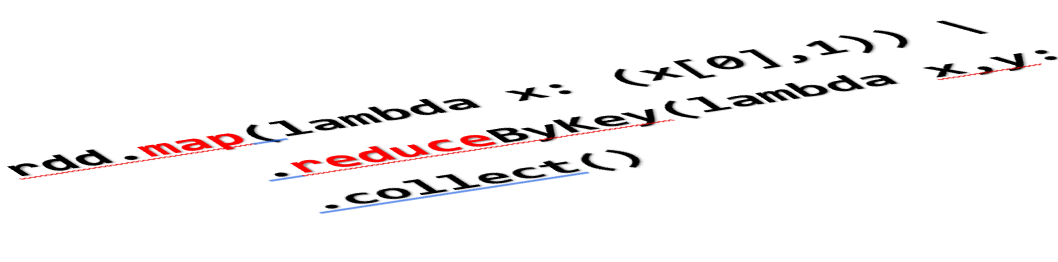
Databricks is a unified data management and analytics platform built by the creators of Apache Spark. It provides a collaborative environment for data scientists, engineers, and business analysts to work together. This brief overview will walk you through the basics of Databricks.

Summary​

Databricks is a cloud-based "as-a-Service" platform for data management and analytics powered by Apache Spark. It enables organizations to deploy scalable, high-performance analytics workloads against large-scale datasets in their cloud environments. Databricks also supports multiple languages (SQL, Python, R, Scala, and Java), interactive notebooks and collaborative features, job scheduling, and more. The Databricks platform supports batch and stream processing and analytics, integrating with various data sources and formats.

Architecture​

The Databricks architecture consists of two main components: the Control Plane and the Data Plane.

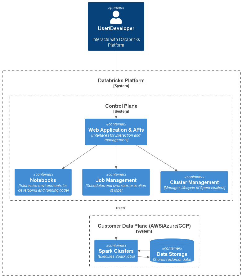
The user interfaces and APIs are located in the Control Plane. It's where users write code in notebooks, manage clusters, and schedule jobs. The Control Plane does not handle customer data directly.

The Data Plane - deployed in the customer's cloud environment and managed by the Control Plane - is where compute clusters (Apache Spark clusters) and storage resources are located. Spark jobs run in the Data Plane to process a customer's data.

This architecture enables a clear separation of responsibilities and increases overall system security. By keeping customer data within the Data Plane, Databricks ensures that sensitive information remains in the customer's environment and control.

Databricks supports a multi-cloud architecture, allowing customers to choose between AWS, Azure, and Google Cloud as their preferred environment for the Data Plane.

Clusters​

Databricks allows you to create Spark clusters required to execute notebook code. Clusters can be Job Clusters used mainly for non-interactive or scheduled workloads, or All Purpose Clusters which are mainly used for ad-hoc, interactive analysis operations. All-Purpose Clusters are shared clusters that multiple users can run commands on simultaneously. The Databricks Control Plane provides cluster automation, scaling, and collaboration capabilities.

Workspaces and Notebooks​

The Workspace is a personalized space where users can create notebooks, import libraries, and run jobs. Notebooks are documents combining code execution, visualizations, and narrative. They support Python, R, Scala, and SQL. Databricks notebooks are similar to popular notebook environments such as Jupyter Notebooks and Apache Zeppelin Notebooks.

Databricks File System (DBFS)​

DBFS is an abstraction layer on top of scalable object storage and offers the benefits of distributed storage without needing local file I/O. DBFS can be used as a source or target for jobs, and Databricks offers multiple utilities for working with DBFS.

Delta Lake and Lakehouse​

Delta Lake is an open-source project providing ACID transactions, scalable metadata handling, and unifying streaming and batch data processing on top of your existing data lake. It brings reliability to data lakes, and it is fully compatible with Apache Spark APIs.

A Lakehouse is a new kind of data management paradigm combining the benefits of data warehouses and data lakes. It provides a data warehouse's reliability, performance, and transactional capabilities with schema-on-read flexibility and low-cost data lake storage.

Delta Live Tables​

Delta Live Tables represent the state of a streaming dataset, views, or materialized views. Delta Live Tables provide improved data availability, quality, and reliability.

Medallion Architecture​

The Medallion Architecture is a methodology for organizing data in your data lake. This is not a new concept; it has been around for a while in the field of data engineering. The names for the layers might differ (like Raw, Clean, and Refined etc), but the concept remains the same. It provides a guideline to systematically organize the data transformation process, with a clear separation between stages.

The Medallion Architecture is named after the 'bronze', 'silver', and 'gold' stages of refining raw material.

Bronze tables, also known as raw tables, store the raw data ingested from various sources. This data is in its original form and hasn't undergone any transformation or cleaning.

Silver tables contain cleansed and enriched data. This results from applying transformations, such as deduplication and schema normalization, to the bronze data.

Gold tables hold business-level aggregates often used for reporting and dashboarding. This might be like daily active users or revenue by geography and product.

This architecture aims to separate data processing into logical layers and allow different teams to work on each layer independently. The Databricks Lakehouse is designed to support this methodology.

if you have enjoyed this post, please consider buying me a coffee ☕ to help me keep writing!

Firstly, this is not another Hadoop obituary, there are enough of those out there already.

The generalized title of this article has been used as an expression to convey the idea that something old has been replaced by something new. In the case of the expression “the King is dead, long live the King” the inference is that although one monarch has passed, another monarch instantly succeeds him.

In the age of instant gratification and hype cycle driven ‘pump and dump’ investment we are very quick to discard technologies that don’t realise overzealous targets for sales or market share. In our continuous attempts to find the next big thing, we are quick to throw out the last big thing and everything associated with it.

The Reports of My Death Have Been Greatly Exaggerated​

A classic example of this is the notion that Map Reduce is dead. Largely proliferated by the Hadoop obituaries which seem to be growing exponentially with each day.

A common e-myth is that Google invented the Map Reduce pattern, which is completely incorrect. In 2004, Google described a framework distributed systems implementation of the Map Reduce pattern in a white paper named “MapReduce: Simplified Data Processing on Large Clusters.” – this would inspire the first-generation processing framework (MapReduce) in the Hadoop project. But neither Google nor Yahoo! nor contributors to the Hadoop project (which include the pure play vendors) created the Map Reduce algorithm or processing pattern and neither shall any one of these have the rights to kill it.

The origins of the Map Reduce pattern can be traced all the way back to the early foundations of functional programming beginning with Lambda Calculus in the 1930s to LISP in the 1960s. Map Reduce is an integral pattern in all of today’s functional and distributed systems programming. You only need to look at the support for map() and reduce() operators in some of the most popular languages today including Python, JavaScript, Scala, and many more languages that support functional programming.

As far as distributed processing frameworks go, the Map Reduce pattern and its map() and reduce() methods are very prominent as higher order functions in APIs such as Spark, Kafka Streams, Apache Samza and Apache Flink to name a few.

While the initial Hadoop adaptation of Map Reduce has been supplanted by superior approaches, the Map Reduce processing pattern is far from dead.

On the fall of Hadoop...​

There is so much hysteria around the fall of Hadoop, we need to be careful not to toss the baby out with the bath water. Hadoop served a significant role in bringing open source, distributed systems from search engine providers to academia all the way to the mainstream, and still serves an important purpose in many organizations data ecosystems today and will continue to do so for some time.

OK, it wasn’t the panacea to everything, but who said it was supposed to be? The Hadoop movement was hijacked by hysteria, hype, venture capital, over ambitious sales targets and financial engineering – this does not mean the technology was bad.

Hadoop spawned many significant related projects such as Spark, Kafka and Presto to name a few. These projects paved the way for cloud integration, which is now the dominant vector for data storage, processing, and analysis.

While the quest for world domination by the Hadoop pure play vendors may be over, the Hadoop movement (and the impact it has had on the enterprise data landscape) will live on.

if you have enjoyed this post, please consider buying me a coffee ☕ to help me keep writing!

Change Data Capture (CDC) is one of the most challenging processing patterns to implement at scale. I personally have had several cracks at this using various different frameworks and approaches, the most recent of which was implemented using Spark – and I think I have finally found the best approach. Even though the code examples referenced use Spark, the pattern is language agnostic – the focus is on the approach not the specific implementation (as this could be applied to any framework or runtime).

The first challenge you are faced with, is to compare a very large dataset (representing the current state of an object) with another potentially very large dataset (representing new or incoming data). Ideally, you would like the process to be configuration driven and accommodate such things as composite primary keys, or operational columns which you would like to restrict from change detection. You may also want to implement a pattern to segregate sensitive attributes from non-sensitive attributes.

Overview​

This pattern (and all my other recent attempts) is fundamentally based upon calculating a deterministic hash of the key and non-key attribute(s), and then using this hash as the basis for comparison. The difference between this pattern and my other attempts is in the distillation and reconstitution of data during the process, as well as breaking the pattern into discrete stages (designed to minimize the impact to other applications). This pattern can be used to process delta or full datasets.

A high-level flowchart representing the basic pattern is shown here:

The Example​

The example provided uses the Synthetic CDC Data Generator application, configuring an incoming set with 5 uuid columns acting as a composite key, and 10 random number columns acting as non key values. The initial days payload consists of 10,000 records, the subsequent days payload consists of another 10,000 records. From the initial dataset, a DELETE operation was performed at the source system for 20% of records, an UPDATE was performed on 40% of the records and the remaining 40% of records were unchanged. In this case the 20% of records that were deleted at the source, were replaced by new INSERT operations creating new keys.

After creating the synthesized day 1 and day 2 datasets, the files are processed as follows:

$ spark-submit cdc.py config.yaml data/day1 2019-06-18
$ spark-submit cdc.py config.yaml data/day2 2019-06-19

Where config.yaml is the configuration for the dataset, data/day1 and data/day2 represent the different data files, and 2019-06-18 and 2019-06-19 represent a business effective date.

The Results​

You should see the following output from running the preceding commands for day 1 and day 2 respectively:

Day 1:​

Day 2:​

A summary analysis of the resultant dataset should show:

Pattern Details​

Details about the pattern and its implementation follow.

Current and Historical Datasets​

The output of each operation will yield a current dataset (that is the current stateful representation of a give object) and a historical dataset partition (capturing the net changes from the previous state in an appended partition).

This is useful, because often consumers will primarily query the latest state of an object. The change sets (or historical dataset partitions) can be used for more advanced analysis by sophisticated users.

Type 2 SCDs (sort of)​

Two operational columns are added to each current and historical object:

• OPERATION : Represents the last known operation to the record, valid values include :
  • I (INSERT)
  • U (UPDATE)
  • D (DELETE – hard DELETEs, applies to full datasets only)
  • X (Not supplied, applies to delta processing only)
  • N (No change)
• EFF_START_DATE

Since data structures on most big data or cloud storage platforms are immutable, we only store the effective start date for each record, this is changed as needed with each coarse-grained operation on the current object. The effective end date is inferred by the presence of a new effective start date (or change in the EFF_START_DATE value for a given record).

The Configuration​

I am using a YAML document to store the configuration for the pattern. Important attributes to include in your configuration are a list of keys and non keys and their datatype (this implementation does type casting as well). Other important attributes include the table names and file paths for the current and historical data structures.

The configuration is read at the beginning of a routine as an input along with the path of an incoming data file (a CSV file in this case) and a business effective date (which will be used as the EFF_START_DATE for new or updated records).

Processing is performed using the specified key and non key attributes and the output datasets (current and historical) are written to columnar storage files (parquet in this case). This is designed to make subsequent access and processing more efficient.

The Algorithm​

I have broken the process into stages as follows:

Stage 1 – Type Cast and Hash Incoming Data​

The first step is to create deterministic hashes of the configured key and non key values for incoming data. The hashes are calculated based upon a list of elements representing the key and non key values using the MD5 algorithm. The hashes for each record are then stored with the respective record. Furthermore, the fields are casted their target datatype as specified in the configuration. Both of these operations can be performed in a single pass of each row using a map() operation.

Importantly we only calculate hashes once upon arrival of new data, as the hashes are persisted for the life of the data – and the data structures are immutable – the hashes should never change or be invalidated.

Stage 2 – Determine INSERTs​

We now compare Incoming Hashes with previously calculated hash values for the (previous day’s) current object. If no current object exists for the dataset, then it can be assumed this is a first run. In this case every record is considered as an INSERT with an EFF_START_DATE of the business effective date supplied.

If there is a current object, then the key and non key hash values (only the hash values) are read from the current object. These are then compared to the respective hashes of the incoming data (which should still be in memory).

Given the full outer join:

incoming_data(keyhash, nonkeyhash) FULL OUTER JOIN
current_data(keyhash, nonkeyhash) ON keyhash

Keys which exist in the left entity which do not exist in the right entity must be the results of an INSERT operation.

Tag these records with an operation of I with an EFF_START_DATE of the business effective date, then rejoin only these records with their full attribute payload from the incoming dataset. Finally, write out these records to the current and historical partition in overwrite mode.

Stage 3 - Determine DELETEs or Missing Records​

Referring the previous full outer join operation, keys which exist in the right entity (current object) which do not appear in the left entity (incoming data) will be the result of a (hard) DELETE operation if you are processing full snapshots, otherwise if you are processing deltas these would be missing records (possibly because there were no changes at the source).

Tag these records as D or X respectively with an EFF_START_DATE of the business effective date, rejoin these records with their full attribute payload from the current dataset, then write out these records to the current and historical partition in append mode.

Stage 4 - Determine UPDATEs or Unchanged Records​

Again, referring to the previous full outer join, keys which exist in both the incoming and current datasets must be either the result of an UPDATE or they could be unchanged. To determine which case they fall under, compare the non key hashes. If the non key hashes differ, it must have been a result of an UPDATE operation at the source, otherwise the record would be unchanged.

Tag these records as U or N respectively with an EFF_START_DATE of the business effective date (in the case of an update - otherwise maintain the current EFF_START_DATE), rejoin these records with their full attribute payload from the incoming dataset, then write out these records to the current and historical partition in append mode.

Key Callouts​

A summary of the key callouts from this pattern are:

• Use the RDD API for iterative record operations (such as type casting and hashing)
• Persist hashes with the records
• Use Dataframes for JOIN operations
• Only perform JOINs with the keyhash and nonkeyhash columns – this minimizes the amount of data shuffled across the network
• Write output data in columnar (Parquet) format
• Break the routine into stages, covering each operation, culminating with a saveAsParquet() action – this may seem expensive but for large datsets it is more efficient to break down DAGs for each operation
• Use caching for objects which will be reused between actions

Metastore Integration​

Although I did not include this in my example, you could easily integrate this pattern with a metastore (such as a Hive metastore or AWS Glue Catalog), by using table objects and ALTER TABLE statements to add historical partitions.

Further optimisations​

If the incoming data is known to be relatively small (in the case of delta processing for instance), you could consider a broadcast join where the smaller incoming data is distributed to all of the different Executors hosting partitions from the current dataset.

Also you could add a key to the column config to configure a column to be nullable or not.

Happy CDCing!

Full source code for this article can be found at: https://github.com/avensolutions/cdc-at-scale-using-spark

if you have enjoyed this post, please consider buying me a coffee ☕ to help me keep writing!